
Build And Train GPT From Scratch
From Zero to GPT: Understanding the Core Components of GPT
In this blog, we’ll build a GPT model from scratch using only Python and PyTorch, without relying on any external libraries. We’ll create and train our own GPT model to match the performance of the original GPT-2 and even fine-tune it on custom data.
By the end of this blog, you will have designed and built a smaller version of a GPT architecture using Python and PyTorch. You will also have trained it entirely from scratch on your own dataset, following the same principles used to train OpenAI’s GPT-2 and GPT-3 language models.
What You can expect by the End of This Blog
- Understand GPT Internals: You’ll learn what happens under the hood of GPT and the key mechanisms that make it work.
- Build a GPT Model Step-by-Step: You’ll define and construct the GPT architecture piece by piece and train it on your own dataset.
- Train a Custom GPT Model: By the end, you’ll have a smaller GPT model built using only Python and PyTorch that you can train and fine-tune on your own data.
- Simplify Training and Fine-Tuning: You’ll discover the simplest way to train or fine-tune a GPT-like transformer model without using external libraries
Before starting, it would be good to introduce GPT and how it’s been built
Introducing GPT
At its core, GPT is a language model designed to predict the next token in a sequence based on the given context. In simpler terms, when you provide a question or some context, GPT generates words sequentially from left to right to complete the sequence.
If you’ve used ChatGPT, you might have noticed that it can generate multiple responses for a single prompt. This is because GPT is a probabilistic system, meaning it can produce different answers to the same prompt depending on its internal state and sampling strategy.
It has been build using the technique introduced in the paper Attention is all you Need, If you’re unfamiliar with the workings of transformers and attention mechanisms, which form the backbone of GPT models, I highly recommend checking out my blog that simplifies these concepts and explains how attention works.
GPT is short form of Generative Pretrained Transformer, so Transformer is a Neural Network which actually does all the heavy lifting under the hood.
Let’s start building the GPT Language Model
We will start with Downloading and inspecting the Dataset.
Downloading the Dataset
To train our GPT model, we need a dataset. And we will use the Shakespeare dataset to train our GPT model
!wget https://raw.githubusercontent.com/karpathy/char-rnn/master/data/tinyshakespeare/input.txtLoad and inspect dataset
Let’s load and inspect the dataset to get an understanding of its structure.
# read it in to inspect it
with open('input.txt', 'r', encoding='utf-8') as f:
    text = f.read()

# let's look at the first 1000 characters
print(text[:1000])
For simplicity and to accommodate limited compute resources, we’ll build a character-level language model. This means we’ll tokenize and train the model based on characters instead of word tokens. Training a token-level language model would require significantly more computational power.
Identifying unique characters in the dataset
chars = sorted(list(set(text)))
vocab_size = len(chars)
print(''.join(chars))
print('Total number of unique characters in the dataset:', vocab_size)
!$&’,-.3:;?ABCDEFGHIJKLMNOPQRSTUVWXYZabcdefghijklmnopqrstuvwxyz Total number of unique characters in the dataset: 65
As shown above, the dataset contains 65 unique characters, which include all alphabetical characters, spaces, and some special symbols.
Tokenize the Input text based on characters
We’ll tokenize the text by mapping each character to an integer
# create a mapping from characters to integers
stoi = { ch:i for i,ch in enumerate(chars) }
itos = { i:ch for i,ch in enumerate(chars) }
encode = lambda s: [stoi[c] for c in s] # encoder: take a string, output a list of integers
decode = lambda l: ''.join([itos[i] for i in l]) # decoder: take a list of integers, output a string

print(encode("hii there"))
print(decode(encode("hii there")))
This simple character-level tokenization method works for our purposes, but there are more advanced techniques like SentencePiece by Google and tiktoken by OpenAI, which tokenize based on words and subwords.
We’ll look at all these tokenization techniques latter on but for simplicity and understanding the GPT model in the better way, we will stick to our character level tokenization.
Let’s tokentize the entire dataset
Next, we encode the entire text dataset into integers and store it in a PyTorch tensor.
# let's now encode the entire text dataset and store it into a torch.Tensor
import torch
data = torch.tensor(encode(text), dtype=torch.long)
Splitting data into train and validation sets
Splitting data into 90% training split and 10% validation split
# Let's now split up the data into train and validation sets
n = int(0.9*len(data)) # first 90% will be train, rest val
train_data = data[:n]
val_data = data[n:]
Preparing the Dataset for Training
It’s important to note that we don’t feed the entire training dataset into the transformer model at once. Doing so would be highly inefficient and computationally expensive. Instead, we work with smaller chunks of the dataset.
So when we actually train Transformers on a lot of these datasets we work with chunks on the dataset therefore before training the Transformer we sample random little chunks out of the training set and train on just chunks at a time. These chunks are limited by a maximum length, referred to as the context length or block size. This approach significantly reduces memory requirements while maintaining efficiency.
block_size = 8 # the context window length

x = train_data[:block_size]   # input sequence to the transformer
y = train_data[1:block_size+1]  # output sequence to the transformer (shifted one position) and it's the target for each position in the input
for t in range(block_size):
    context = x[:t+1]
    target = y[t]
    print(f"when input is {context} the target: {target}")
We train on all the eight(block_size) examples here with context size between 1 and context of block_size because we want the transformer model to seeing context all the way from as little as 1 to all the way to block size. And this is really going to useful later during infernece because we can generate text of any length by just giving it a context of any length.
Note: Model can take maximum of block_size context length as input, so during inference when generating text more than block_size length, it will start truncating the context from the beginning. i.e. it take last block_size tokens as input and generate next token and append it to the input and generate next token and so on.
Batch Processing
We will add another dimension to out dataset which is batch size because GPUs are very good at processing data parallely therefor all the inputs in the batch will be process parallelly, that will make the training more efficient.
torch.manual_seed(1337)
batch_size = 4 # how many independent sequences will we process in parallel?
block_size = 8 # what is the maximum context length for predictions?

def get_batch(split, batch_size, block_size):
    # generate a small batch of data of inputs x and targets y
    data = train_data if split == 'train' else val_data
    ix = torch.randint(len(data) - block_size, (batch_size,))
    x = torch.stack([data[i:i+block_size] for i in ix])
    y = torch.stack([data[i+1:i+block_size+1] for i in ix])
    return x, y

xb, yb = get_batch('train', batch_size, block_size)
Self-attention: The basic building block of the Transformer
Now that we have the basic setup for our model, it’s time to dive into one of the key components of the Transformer architecture — self-attention.
Intro: Self-Attention
Self-attention is a mechanism that relates each word in a sentence to every other word, this allows each word to understand its context within the sentence. This process generates final `out_dim` dimention output vector for each word, which captures its relationship with every other word in the sentence.
Key Components: Query, Key, and Value
To compute self-attention, we need three vectors: query, key, and value. These vectors are derived from the word embeddings of each word in the sentence. They are typically smaller in size than the original embeddings. In our case, these vectors are 64-dimensional.
Note: These new vectors are smaller in dimension than the embedding vector.
Query, Key and Values can be interpreted as follows:
- query: what I are looking for (what I are interested in)
- key: what I have
- value: If the key matches what I are looking for, this is the information I want to retrieve
These query, key, and values vectors helps to captures the relationship for each word in a sentence to every other word.
import torch.nn as nn
import torch.nn.functional as F

torch.manual_seed(1337)
batch_size = B = 4 # how many independent sequences will we process in parallel?
block_size = T = 8 # what is the maximum context length for predictions?
embed_dim = C = 32 # embedding dimension of the input tokens

x  = torch.randn(B, T, C) # input tokens

# let's create a single head perform self-attention
head_size = H = 16 # how big is the head (size of the key, query, value projections)
key = nn.Linear(C, head_size) # linear layer for key
query = nn.Linear(C, head_size) # linear layer for query
value = nn.Linear(C, head_size) # linear layer for value

# apply the linear projections to the input tokens x to get the keys, queries and values for all tokens in the batch
k = key(x)   # shape: (B, T, H) (batch size, time steps, head size)
q = query(x)  # shape: (B, T, H)
v = value(x)  # shape: (B, T, H)
Calculating scores in Self-Attention
To calculate self-attention, we compute a score for each word in the sequence. This score is determined by the dot product of the query (q) for a word and the key (k) for every word in the sequence. This score tells us how much attention a word should pay to each token in the sequence, including itself.
Scaling: We scale the dot products by dividing by the square root of the head size. This ensures that the variance of the attention scores remains consistent, preventing saturation during the softmax operation.
# let's compute the raw self-attention scores (a simple dot product between the queries and the keys for all tokens in the batch)

scores_matrix = q @ k.transpose(-2, -1) # (B, T, H) @ (B, H, T) -> (B, T, T) (batch size, time steps, time steps)

# we also divide the scores by the square root of the head_size
# This is because we are scaling the dot products by the head_size, so that the result is not too large and the softmax is not too peaked.
scores_matrix = scores_matrix / torch.sqrt(torch.tensor(H).float()) # shape: (B, T, T)
Masking Scores: Attenting tokens that come before the current token
In language modeling, each token should only attend to the tokens before it in the sequence, not the ones that come after. This prevents the model from peeking at future tokens when predicting the current token.
This is a specific case of language modeling, where we want to mask out the upper half of the matrix, so that future tokens cannot communicate with the past tokens.
This is done by masking the upper half of the scores matrix, ensuring that the model cannot attend to future tokens. After masking, we apply the softmax function to the scores matrix.
Also note that this is not a constraint for general case of self-attention mechanism there are many other usecase where we don’t want to mask the matrix like in case of translation task we want to allow the future tokens to communicate with the past tokens and other use cases like sentence classification etc.
mask = torch.tril(torch.ones(T, T))
mask_score_matrix = scores_matrix.masked_fill(mask == 0, float('-inf')) # masking out the upper half of the matrix #shape: (B, T, T)

print(f"mask_score_matrix shape: {mask_score_matrix.shape}")

print(mask_score_matrix[0])
Calculating attention weights using Softmax
Now we apply the softmax function to the scores matrix to get the attention weights, with the softmax applied on the last dimension (time dimension) of the scores matrix we will get the attention weights for each token in the sequence to all other tokens in the sequence.
attention_weights = F.softmax(mask_score_matrix, dim=-1) # shape: (B, T, T)

print(f"shape of the attention weights: {attention_weights.shape}")

print(f"Sum of the attention weights for each token in the batch: {attention_weights.sum(dim=-1)}")
Output of the self-attention mechanism in single head setting
Output of the self-attention mechanism is computed by a weighted sum of the values for all tokens in the batch, which are weighted by the attention weights.
This can effectively be computed by a matrix multiplication of the attention weights with the values.
# now we compute the output of the self-attention layer by multiplying the attention weights with the values
attention_output = attention_weights @ v # shape: (B, T, T) @ (B, T, H) -> (B, T, H) (batch size, time steps, head size)

print(f"shape of the attention output: {attention_output.shape}")
Let’s put everything together in a single nn.Module
Self-Attention Head
class SelfAttentionHead(nn.Module):
    """ one head of self-attention """

    def __init__(self, embed_dim, block_size, head_size, dropout=0.2):
        super().__init__()
        self.key = nn.Linear(embed_dim, head_size, bias=False)
        self.query = nn.Linear(embed_dim, head_size, bias=False)
        self.value = nn.Linear(embed_dim, head_size, bias=False)
        self.register_buffer('tril', torch.tril(torch.ones(block_size, block_size)))

        self.dropout = nn.Dropout(dropout)

    def forward(self, x):
        # input of size (batch, time-step, channels)
        # output of size (batch, time-step, head size)
        B,T,C = x.shape
        k = self.key(x)   # (B,T,hs)
        q = self.query(x) # (B,T,hs)
        # compute attention scores ("affinities")
        wei = q @ k.transpose(-2,-1) * k.shape[-1]**-0.5 # (B, T, hs) @ (B, hs, T) -> (B, T, T)
        wei = wei.masked_fill(self.tril[:T, :T] == 0, float('-inf')) # (B, T, T)
        wei = F.softmax(wei, dim=-1) # (B, T, T)
        wei = self.dropout(wei)
        # perform the weighted aggregation of the values
        v = self.value(x) # (B,T,hs)
        out = wei @ v # (B, T, T) @ (B, T, hs) -> (B, T, hs)
        return out
Additional Informantion about Attentions
- Attention is a **communication mechanism**. Can be seen as nodes in a directed graph looking at each other and aggregating information with a weighted sum from all nodes that point to them, with data-dependent weights.
- There is no notion of space. Attention simply acts over a set of vectors. This is why we need to positionally encode tokens.
- Each example across batch dimension is of course processed completely independently and never “talk” to each other
- “self-attention” just means that the keys and values are produced from the same source as queries. In “cross-attention”, the queries still get produced from x, but the keys and values come from some other, external source (e.g. an encoder module)
Multi-Head Attention
Multi-head attention is just calculating multiple self-attention heads in parallel and then concatenating their results. And this help the model to learn different representation of the input data.
class MultiHeadSelfAttention(nn.Module):
    """ a stack of self-attention layers """

    def __init__(self, embed_dim, block_size, num_heads, head_size, dropout=0.2):
        super().__init__()
        self.heads = nn.ModuleList([SelfAttentionHead(embed_dim, block_size, head_size, dropout) for _ in range(num_heads)])
        self.projection = nn.Linear(num_heads*head_size, embed_dim)
        self.dropout = nn.Dropout(dropout)


    def forward(self, x):
        # input of size (batch, time-step, channels)
        # output of size (batch, time-step, channels)
        head_out = [head(x) for head in self.heads] # a list of tensors of shape (B, T, hs)
        out = torch.cat(head_out, dim=-1) # concatenate along the feature dimension
        out = self.projection(out) # project back to the original feature dimension
        out = self.dropout(out)
        return out
Positional Encoding
Irrespective of RNNs where word tokens are input one at a time into the model, whereas in the attention model, all the words are input at the same time i.e. all the words taken as input parallelly into the encoder model. And the position and order of words are essential parts of any language since they define the grammar and thus the actual semantics of a sentence. So, we need to do something to maintain the order of sequence therefore, to provide the model with positional information we add positional encoding to the input embeddings.
Positional encoding is a way to inject some information about the relative or absolute position of the tokens in the sequence. The positional encoding vector is added to the embedding vector. Embeddings represent a token in a d-dimensional space where tokens with similar meaning will be closer to each other. But the embeddings do not encode the relative position of words in a sentence. So after adding positional encoding, words will be closer to each other based on the similarity of their meaning and their position in the sentence, in the d-dimensional space.
import math

# Position embeddings
class PositionalEncoding(nn.Module):
    def __init__(self, embed_dim, max_len=5000):
        super().__init__()
        # Compute the positional encodings once in log space.
        pe = torch.zeros(max_len, embed_dim)
        position = torch.arange(0, max_len).unsqueeze(1).float()
        div_term = torch.exp(torch.arange(0, embed_dim, 2).float() * -(math.log(10000.0) / embed_dim))
        pe[:, 0::2] = torch.sin(position * div_term)
        pe[:, 1::2] = torch.cos(position * div_term)
        pe = pe.unsqueeze(0)
        self.register_buffer('pe', pe)

    def forward(self, x):
        return x + self.pe[:, :x.size(1)]
Feed forward network
This is a simple feed-forward network with a simple liner layer followed by non-linear activation functions that is applied to each positional token separately and identically.
This helps the model learn more complex functions than just the linear ones that self-attention provides.
# Feed forward network
# hidden_dim is 4 times the embedding dimension as per the paper "Attention is all you need"

class FeedForward(nn.Module):
    def __init__(self, embed_dim, hidden_dim, dropout=0.2):
        super().__init__()
        self.net = nn.Sequential(
            nn.Linear(embed_dim, hidden_dim),
            nn.ReLU(),
            nn.Linear(hidden_dim, embed_dim),
            nn.Dropout(dropout)
        )

    def forward(self, x):
        return self.net(x)
Putting it all together in a Transformer Block
Transformer Block
The transformer block is composed of a multi-head self-attention layer, followed by a feed-forward network.
# Putting it all together in a transformer block
# The transformer block is composed of a multi-head self-attention layer, followed by a feed-forward network.

class TransformerBlock(nn.Module):
    def __init__(self, embed_dim, block_size, num_heads, head_size, ff_hidden_dim, dropout=0.2):
        super().__init__()
        self.attention = MultiHeadSelfAttention(embed_dim, block_size, num_heads, head_size, dropout)
        self.ffn = FeedForward(embed_dim, ff_hidden_dim)

    def forward(self, x):
        x = self.pos_emb(x)
        x = self.attention(x)
        x = self.ffn(x)
        return x
Skip connections in Transformer Block
Adding skip connections around the multi-head self-attention and feed-forward network is crucial for training a very deep model.
Without skip connections, the gradients tend to either vanish (in very deep feed-forward networks) or explode (in very deep networks with attention). Therefore, skip connections are crucial for training very deep models.
We add a residual connection around the multi-head self-attention and feed-forward network, followed by layer normalization. We first look at the skip connection and then at the layer normalization.
# Skip connections

class TransformerBlock(nn.Module):
    def __init__(self, embed_dim, block_size, num_heads, head_size, ff_hidden_dim, dropout=0.2):
        super().__init__()
        self.attention = MultiHeadSelfAttention(embed_dim, block_size, num_heads, head_size, dropout=dropout)
        self.ffn = FeedForward(embed_dim, ff_hidden_dim)


    def forward(self, x):
        x = self.pos_emb(x)  # shape (B, T, C)
        # apply the self-attention mechanism
        att = self.attention(x) # shape (B, T, C)
        # add skip connection
        x = x + att
        # apply the feed-forward network
        ffn = self.ffn(x)  # shape (B, T, C)
        # add skip connection
        x = x + ffn  # shape (B, T, C)
        return x
Transformer Block with Layer Normalization
This helps stabilize the training of deep networks and speeds up convergence by normalizing the pre-activation outputs of each layer.
In the orignal paper, Layer normalization is applied to the output of the self-attention and the feed-forward network but now generally it is applied to the input of the self-attention and the feed-forward network and not the output.
class TransformerBlock(nn.Module):
    def __init__(self, embed_dim, block_size, num_heads, head_size, ff_hidden_dim, dropout=0.2):
        super().__init__()
        self.attention = MultiHeadSelfAttention(embed_dim, block_size, num_heads, head_size, dropout=dropout)
        self.norm1 = nn.LayerNorm(embed_dim)
        self.ffn = FeedForward(embed_dim, ff_hidden_dim)
        self.norm2 = nn.LayerNorm(embed_dim)

    def forward(self, x):
        # apply the self-attention mechanism
        att = self.attention(x) # shape (B, T, C)
        # add skip connection and apply layer normalization
        x = x + self.norm1(att)
        # apply the feed-forward network
        ffn = self.ffn(x)  # shape (B, T, C)
        # add skip connection and apply layer normalization
        x = x + self.norm2(ffn)
        return x
GPT Model Architecture
Let’s now create a decoder based GPT transformer model composed of multiple transformer blocks
class GPTLanguageModel(nn.Module):
    def __init__(self, vocab_size,embed_dim, block_size, num_heads, head_size, ff_hidden_dim, num_layers, dropout=0.2):
        super().__init__()
        self.emd = nn.Embedding(vocab_size, embed_dim)
        self.pos_emb = PositionalEncoding(embed_dim)
        self.layers = nn.ModuleList([
            TransformerBlock(embed_dim, block_size, num_heads, head_size, ff_hidden_dim, dropout=dropout)
            for _ in range(num_layers)
        ])
        self.norm = nn.LayerNorm(embed_dim)
        self.head = nn.Linear(embed_dim, vocab_size)

    def forward(self, x):
        x = self.emd(x)
        x = self.pos_emb(x)
        for layer in self.layers:
            x = layer(x)
        x = self.norm(x)
        x = self.head(x)
        return x
Model Initialization
We will now intiatilze our model with different model settings and calculate number of training parameters at the end
# Model Initialization and Number of Parameters

torch.manual_seed(1337)

# model hyperparameters
chars = sorted(list(set(text)))
vocab_size = len(chars)
embed_dim = 384
num_heads = 6
head_size = 64
ff_hidden_dim = 4*384
num_layers = 6
block_size = 256
dropout = 0.3

model = GPTLanguageModel(vocab_size, embed_dim, block_size, num_heads, head_size, ff_hidden_dim, num_layers, dropout=dropout)

device = torch.device("cuda" if torch.cuda.is_available() else "cpu")

model = model.to(device)

# Number of parameters in the model
num_params = sum(p.numel() for p in model.parameters())

print(f"Number of parameters in the model: {num_params}")
Let’s Train Our GPT Transformer Model
# Let's now train our transformer model
# we will use the cross-entropy loss and the Adam optimizer to train the model.

device = torch.device('cuda' if torch.cuda.is_available() else 'cpu')
print(f"Training on device {device}.")

# training parameters
lr = 3e-4
batch_size = 64
num_iterations = 3000
eval_iters = 200

# intiatizing loss and optimizer
criterion = nn.CrossEntropyLoss()
optimizer = torch.optim.Adam(model.parameters(), lr=lr)

@torch.no_grad()
def estimate_loss(model, criterion, eval_iters, batch_size, block_size):
    model.eval()
    out = []
    losses = torch.zeros(2, eval_iters)

    @torch.no_grad()
    def evaluate(model, criterion, batch_size, block_size):
        model.eval()
        out = []
        with torch.no_grad():
            for split in ['train', 'val']:
                x, y = get_batch(split, batch_size, block_size)
                x, y = x.to(device), y.to(device)
                y_pred = model(x)
                loss = criterion(y_pred.view(-1, vocab_size), y.view(-1))
                out.append(loss.item())
        return out

    for i in range(eval_iters):
        losses[0, i], losses[1, i] = evaluate(model, criterion, batch_size, block_size)
    return losses.mean(dim=1).tolist()


# training function
def train(model, criterion, optimizer, num_iterations, batch_size, block_size):
    model.train()
    losses = []

    output_losses = []
    for i in range(num_iterations):
        x, y = get_batch('train', batch_size, block_size)
        x, y = x.to(device), y.to(device)
        optimizer.zero_grad()
        y_pred = model(x)  # shape (B, T, vocab_size)
        loss = criterion(y_pred.view(-1, vocab_size), y.view(-1))
        loss.backward()
        optimizer.step()
        losses.append(loss.item())
        if i % eval_iters == 0:
            # mean training loss over the last 100 batches
            mean_train_loss = sum(losses[-eval_iters:]) / float(eval_iters)

            print(f'iteration {i}, mean training loss: {mean_train_loss:.2f}')

            train_loss, val_loss = estimate_loss(model, criterion, eval_iters, batch_size, block_size)
            output_losses.append((train_loss, val_loss))
            print(f'train loss: {train_loss:.2f}, val loss: {val_loss:.2f}')

    return output_losses

losses = train(model, criterion, optimizer, num_iterations, batch_size, block_size)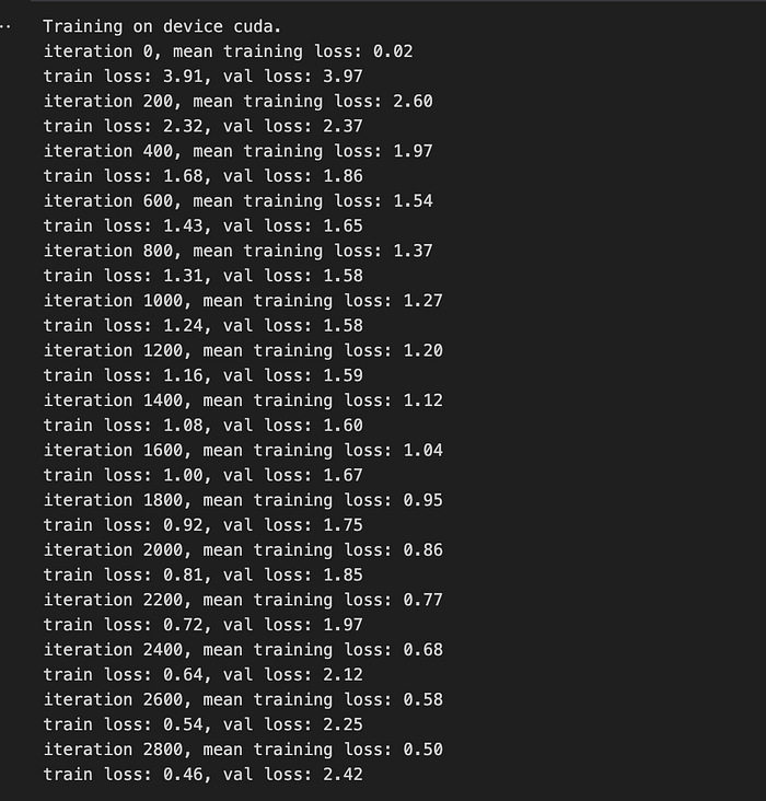
Virsualizing the Training and Validation losses
Seeing the training and validation loss over time we can see that the model is learning and the validation loss is decreasing over time for a certain point but after that validation loss starts to increase again. This is a sign of overfitting.
import matplotlib.pyplot as plt

train_loss, val_loss = zip(*losses)

plt.figure(figsize=(10, 5))
plt.plot(train_loss, label='train loss')
plt.plot(val_loss, label='val loss')
plt.xlabel('iterations')
plt.ylabel('loss')
plt.legend()
plt.show()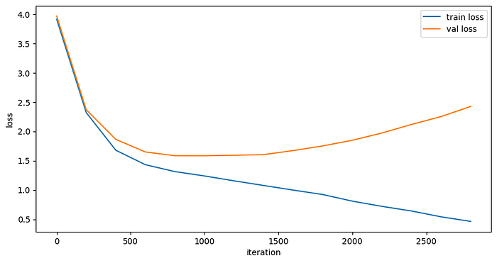
Generation from Trained Model
Let’s now generate some text using the trained transformer mode
@torch.no_grad()
def generate_text(model, input, max_new_tokens = 100, temperature = 1.0):
    model.eval()

    out = ''
    if isinstance(input, str):
        input = encode(input)
    input = torch.tensor(input, dtype=torch.long, device=device).unsqueeze(0)
    for _ in range(max_new_tokens):
        with torch.no_grad():
            input = input[:, -block_size:]
            y = model(input)  # shape (B, T, vocab_size)
            # take the logits at the final time-step and scale by the temperature
            y = y[0, -1, :] / temperature  # shape (vocab_size,)
            y = torch.softmax(y, dim=-1)
            next_token = torch.multinomial(y, 1)
            # if next_token == 0:
            #     break
            print(decode([next_token.item()]), end='', flush=True)
            out += decode([next_token.item()])
            input = torch.cat((input, next_token.unsqueeze(0)), dim=1)
    return out

generate_text(model, "The", max_new_tokens=1000, temperature=0.8)
Output

Conclusions
Building and training a GPT model from scratch is a rewarding yet challenging journey. By delving deep into the mechanics of transformers, self-attention, and multi-head attention, we’ve gained a solid understanding of what powers large language models like GPT-2 and GPT-3. Piece by piece, we constructed the GPT architecture, trained it on custom data, and observed its capabilities in text generation.
Key Takeaways from Building GPT from Scratch
- Deep Understanding of GPT Internals: You now have a clear understanding of the internal mechanics of GPT models, including how self-attention, multi-head attention, and transformer blocks work.
- Hands-on Experience: Successfully built a smaller version of a GPT model using only Python and PyTorch, starting from basic components.
- Practical Knowledge of Training: Learned how to train and fine-tune a GPT model on your own dataset using simplified methodologies.
Future Work
- Improve the overall performance of the model using hyperpamaters, AdamW, gradient clipping, etc
- Improve the validation loss and reduce overfitting using hyperpamaters, learning rate scheduler, etc
- Optimize the inference speed using different optimizations like torch.compile, kernel fusion, flash attention, float16 conversion, etc.
- Optimize training speed — distributed data parallel (DDP), LORA, etc.
References
Neural Networks: Zero to Hero by Andrej Karpathy — YT playlist
Attention Is All You Need — Research Paper